Can cable sound be measured? A €2.800 USB cable put to the studio test.

Is there such a thing as cable sound, or is it just a narrative? We connected two USB cables, each costing €2.800, to our studio chain, measured the entire transmission, and then listened to 20 rounds of blind listening. Here are all the figures, all the limits – and what cannot be deduced from them.

Transparency notice (advertising): VBS Audio provided us with two cables of the model “Eigen” free as a product sample The materials were provided. No money changed hands, there was no compensation, and no agreement was made regarding the outcome. The manufacturer granted permission for the publication of photos, company name, and website and agreed to the procedure in advance. We consistently distinguish between manufacturer specifications, our own measurements, and subjective listening impressions in the text.

Cable sound Digital audio cables have been a contentious issue in the hi-fi and studio world for decades – and one that's almost always debated without numbers. The discussion is particularly heated when it comes to digital audio cables, such as USB, coaxial, Toslink, or AES. A manufacturer contacted us: their cables made an audible difference, especially at the digital level. We agreed – on one condition: we would measure the entire chain, conduct blind listening tests, and publish everything, regardless of the outcome. This report is the result, with all the figures, all the limitations, and everything else we learned. not can say.

Contents of this cable sound test

Is there such a thing as cable sound? We measured it in the studio.

Cable sound refers to the assumption that different cables audibly alter the same signal path. This was not demonstrable in this series of measurements. Under the documented conditions, neither a consistent subjective preference nor a uniformly better fidelity to the original sound emerged for either of the two cable configurations. Small numerical deviations were measurable; however, in this setup, they cannot be definitively attributed to the USB cables. Therefore, this finding pertains to two specific cables in a specific chain, but it does not constitute a general conclusion.

Cable sound in five points: the result

  • Digital transmission: Initially, the data arrived flawlessly at the 24-bit level in the tested sections – with the test cable just as with the original cable. The USB error counters of the RME interfaces remained at zero during the documented endurance tests.
  • Frequency Response: Furthermore, both states overlap across the entire audible range except for less than 0,0002 dB.
  • Music signal: Furthermore, the residual waveform difference between the conditions is approximately -109,9 to -109,4 dBFS – practically on the same order of magnitude as the variation between two recordings the same condition.
  • The only noticeable deviation: Only in the noise band during silence was the reference condition around +0,104 dB (left) / +0,116 dB (right) higher. There is only one silent image per condition – this does not provide any information about the cause.
  • Blind preference screening: Finally, 20 rounds, one listener, 11 winning votes for the VBS cable, 9 for the RME cableThe two-sided exact binomial test against 50:50 yields p = 0,824.

Why we go to this trouble: We work in mastering Every day, we encounter differences that lie at the edge of perception. Anyone who wants to separate claims from findings must measure and listen in blinded conditions – otherwise, the price tag will be a deciding factor. And most importantly, because it's almost always misquoted: A non-significant result is not proof of sound equality. The test examined a preference – not whether someone can reliably distinguish between the two states. These are two different questions, and we only answered one of them.

How it came about: an offer for a cable sound test

First, some background: The manufacturer contacted me – a small-scale manufacturer, not a mass-produced product. We spoke on the phone, he told me a lot about his cables and his company's history, and, as I recorded on tape immediately after the test day, "Also always touted as making a huge difference, especially in the digital realm, by using such cables.".

Why do we even test audiophile USB cables?

My answer was therefore: gladly, but properly. I offered a comprehensive test scenario, including a blog post and complete results, including technical measurements and blind listening sessions. Open-ended.

My voice note also explains why I participated at all, even though I am skeptical of such statements:

"Since I myself am still very skeptical of such statements, because so much is always said about it, these typical audio myths. And yes, now we really have a manufacturer who actually knows what he's talking about, and where we simply want to check it out and see: what really comes out of it."

Why we agreed to the cable sound test

That's precisely the point. The issue of cable sound has been debated for twenty years, almost always without any concrete data. However, we have a studio, measuring equipment, and the capability to conduct a clean, blind test. So we're doing it – just as we usually try to... To test common assumptions about studio work in practice.
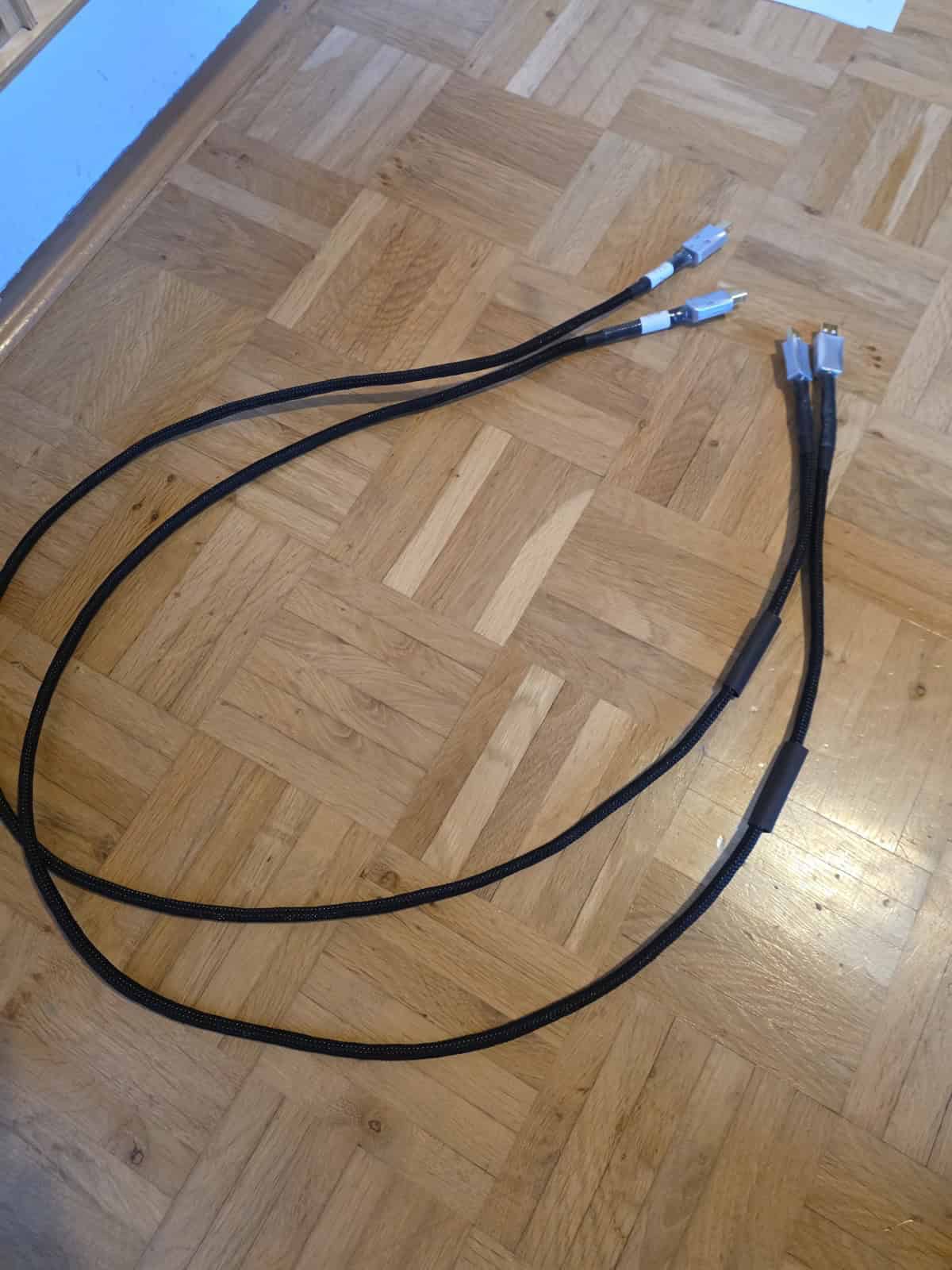
Cable sound test: two VBS Audio Eigen USB cables with fabric sheathing on a parquet floor
The two test samples: VBS Audio Eigen, 1,5 m each, USB-A to USB-B. Fabric sheath, screwed metal housings, gold-plated contacts. Photo: Peak-Studios.

The product: an audiophile USB cable from the manufacturer

First, the facts about the test subject. Everything in this section is manufacturer's instructionsThey are not the result of our measurements, and we have not verified them – that is not possible with the methods used here.

ModelVBS Audio Own
Length1,5 m
SpecificationUSB 2.0 high speed (480 Mbit/s)
List price€2.000 base for the first meter; €2.800 for 1,5 m
Pricing logicnon-linear – each additional step of 0,5 m adds 40% to the initial length (2 m would therefore correspond to €3.920)
SalesExclusively direct, limited quantity, no distribution in Germany

Price as of August 2026, written information from the manufacturer. Anyone considering purchasing should inquire about the current price directly with the manufacturer. vbsaudio.com.

What the manufacturer says about the construction

Conductor material, microstructure, geometry, shielding and connector termination are considered an integrated system Developed. Details regarding shielding, grounding, and internal construction are confidential and will not be disclosed; therefore, the evaluation should refer to the finished cable. The manufacturer also requests that the product be presented as a "precision calibration/reference system tool" and emphasizes "signal integrity in the time domain."

Fair assessment of these theses

  • Our measurements neither confirm nor refute the mechanisms mentioned. We did not perform any material analysis, high-frequency measurements on the line, or calibrated jitter measurements. Anyone wanting to test this needs a measurement setup that can do exactly that.
  • Regarding time behavior: The devices in this chain operate asynchronously – the converter clocking comes from the device itself, not from the USB connection. The ADI-2 Pro ran on... Clock Source InternalThat's an argument, but not a measurement from us, and it doesn't rule out mass or shielding effects.
  • To play: According to the manufacturer, the cables are already broken in, but the sound can "open up further." The cables had been installed in the studio for about two to three weeks on the day of the measurement – ​​this is my own statement regarding usage, not a controlled verification. A proper before-and-after test would have to include an unaltered reference run; otherwise, you'd be measuring device temperature and contact condition. We didn't do that here.
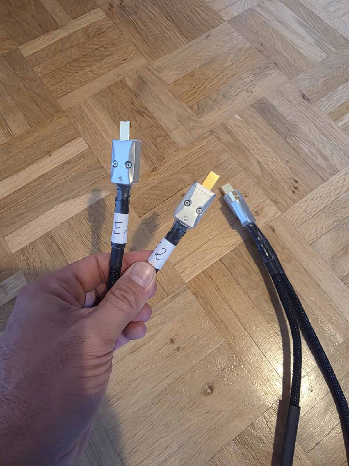
Cable sound test sample: Close-up of the USB-B connectors with the markings E1 and E2
For traceability, both samples were labeled E1 and E2. The standard RME cable is shown on the right as a reference. Photo: Peak-Studios.

Cable sound with digital audio cables: four approaches, four discussions

First, a clarification: People who talk about digital audio cables rarely mean the same thing. In the studio, four transmission paths operate simultaneously, and they differ significantly from each other technically. This is important because the results of this test not automatically transferred to each of these paths.

send email nowTypical applicationClockingWhat is being discussed here
USBComputer to audio interfaceasynchronous – the device clocks itselfGrounding, shielding, interference in the analog stages
AES3 / AES-EBUInterface to converter or active loudspeakerClock signal embedded in the signal, 110 ohms balancedImpedance matching, reflections due to incorrect cable type
S/PDIF coaxialConsumer devices, older convertersClock signal is embedded in the signal, 75 ohms unbalancedImpedance, ground connection between two devices
Optical ToslinkConsumer devices, galvanic isolationThe clock signal is embedded in the signal.Light scattering and slope steepness over long distances

Cable sound in hi-fi and in the studio: the same debate, different conditions

The discussion about cable sound is primarily conducted in the high-end hi-fi sector, and there it usually revolves around speaker cables and power cords. Both are analog connections: Cross-section, length, capacitance, and inductance determine measurable electrical properties, and in the case of speaker cables, the behavior also depends on the impedance of the connected speaker. Whether this translates into a sonically relevant difference in a specific case is a separate question – but the physical basis for it exists.

With a digital connection, however, things are different. Here, no music signal is transmitted, but rather a data stream. A single cable in a streaming or studio system cannot therefore sound "warmer"—it can either transmit the data correctly, or it can introduce errors. That's precisely why we tested both levels separately in this review: first the data transmission, then the analog output.

Furthermore, the quality of the connectors must be considered: Poorly fitting or oxidized connectors create intermittent connections – and these manifest as dropouts, not as tonal characteristics. The connectors of the test samples fit snugly and are screwed in, which is a more practically relevant advantage in everyday studio use than any claim regarding sound quality.

Why cable sound is evaluated differently with USB

Consequently, the crucial difference lies in the rhythm: At USB in asynchronous mode The clock in the device determines the conversion time, not the incoming signal. With AES3, coaxial, and Toslink, however, the clock is embedded in the data stream itself – in these cases, the discussion about cable influences is technically better justified because impedance errors and reflections can blur the signal edges.

Therefore, our test focuses exclusively on the USB connection. It says nothing about cable sound quality with coaxial or optical digital audio cables. Anyone suspecting problems there should first check the impedance of the cable used – a 75-ohm video cable behaves differently on an S/PDIF input than any random RCA cable from a drawer.

And another point that is often missing in cable discussions: A defective or borderline cable can This can indeed have audible consequences – however, with digital transmission, this doesn't manifest as a "warmer sound," but rather as dropouts, crackling, or connection interruptions. That's precisely why we logged the error counters.

Instead of speculating about cables: Let us hear where your mix really stands.
We'll tell you exactly what reserves are in your production.

The test bench: where cable sound could originate

First, one must distinguish between two things: what was recorded and what was overheardThese are different approaches for us.

Recorded signal path of the analog measurements

Identical in both cable states. Only the two red-marked USB connections were changed – and both were changed simultaneously.

Computer and test object

DAW computerCubase, 44,1 kHz, 32-bit float
Test object 1 · USB cableVBS proprietary (USB 2) vs. RME original (USB 2)on the ADI-2 Pro – same USB mode
RME ADI-2 Pro FS R BEDigital/analog conversion and backClock source: internal, separate power supply

Recording loop in the project

Music trackMontez “a person with a heart”Excerpt 60,666 seconds
"Analog" groupExternal effect “Analog chain”Send 0,00 dB
Analog outputConversion to analog
XLR and PatchbayFlock Audio, Path 23 left / 24 rightdirectly, without any connected devices
Analog inputConversion back to digital
Return to the groupReturn 0,00 dB
Recording track “Final Mix”44,1 kHz · Stereo · 32-bit float · five complete passes per stateAdditionally: silence, 1 kHz sine wave, sweep from 20 Hz to 20 kHz

Eavesdropping path – separate from recording path

DAW computerAcourate Convolver, equalization via filter
Test object 2 · USB cableVBS proprietary (USB 2) vs. RME original (USB 3)on the UFX+ – here the cable and operating mode change together
RME Fireface UFX+AES3 digital output
Dutch & Dutch 8Ctwo active speakersConversion to analog in the loudspeaker

Clock chain: The ADI-2 Pro (internal) passes the clock signal to the UFX+, which runs synchronously at 44,1 kHz. The recorded path includes XLR connections, the patchbay path, and both converter stages of the ADI-2 Pro. This is explicitly not an isolated cable, converter, or jitter measurement.

The admission process

Initially, the music track in Cubase is routed to a group called "Analog". There, a External Effect (Analog chain) with send and return set to exactly 0,00 dB. The signal passes through the analog output of the RME ADI-2 Pro FS R Black Edition Beyond that, via XLR and a direct path from the Flock Audio patchbay (23 L / 24 R, without any inserted processors) back to the analog input of the same device and from there to the recording track "Final Mix" – 44,1 kHz, stereo, 32-bit float. The fact that the send and return are set to exactly unity gain is not a detail, but a prerequisite for any comparison – nothing other than consistent... clean level management in the signal chain.

Cubase dialog External effects with Send Gain 0,00 dB and Return Gain 0,00 dB for the analog measurement loop
Methodological evidence: The send and return of the external effect are set to exactly 0,00 dB. Previously, they were -6 dB / +6 dB; the change was saved before the first take and read in the program window.

The eavesdropping route

This one, however, runs completely separately: Cubase → Acourate Convolver (FIR equalization) → RME Fireface UFX+ → AES3 → left Dutch & Dutch 8C → AES-THRU → right 8C. The digital-to-analog conversion for monitoring therefore takes place in the speakers, not in the interface.

What exactly was changed – and why that limits the cable sound assessment.

Finally, both USB connections, namely together in one operation.

GerätReference stateTest conditionPlease note:
ADI-2 Pro FS R BERME standard cable, USB 2VBS Eigen E1, USB 2clean cable comparison in the same mode
Fireface UFX+included RME cable, USB 3VBS Eigen E2 USB 2Cables and Switch operating modes here

This is a conscious decision and at the same time the most important limitation of the structure: The UFX+ branch is a Practical comparison: Delivered state versus test cableThis isn't just a cable comparison. RME ships the UFX+ with a USB 3 cable – nobody would swap that for a USB 2 cable in everyday use just for the sake of comparison. The manufacturer would have preferred the same setup; we opted for the real-world configuration and are disclosing that here. The device's technical specifications are listed in the ADI-2 Pro FS R manual.

Consequence for the evaluation: Since both cables were replaced together, the analog recordings are compared. two combined system statesThis does not causally isolate a single cable or interface. The recorded path also includes XLR connections, the patchbay path, and both converter stages of the ADI-2 Pro. It is not an isolated converter, cable, or jitter measurement—similar to comparing... analog hardware versus plugins, where you always measure the entire chain and never just one component.

Beforehand, everything was backed up: project copy, Cubase configuration, patchbay and mixer files, screenshots of the initial state, and a manifest with SHA-256 checksums. The raw recordings were checked again after recording and were neither normalized, edited, nor overwritten.

Digital transmission: the precursor to every cable sound question

First of all, the first question was already answered before the day of measurement: Will the data arrive intact? These tests were conducted before the measurement day and were already documented.

Bit test on the ADI-2 Pro

First, the bit test: The ADI-2 Pro can check in its device menu whether a test signal is received with bit-perfect accuracy. The result was identical with both the reference cable and the test cable: 16-bit file "16 bits passed", 24-bit file "24 bits passed". With the 32-bit file, the device displayed... both In some cases, only "24 bits passed" was displayed. This documents the resolution limit of the tested playback path. no 32-bit pass and no cable faultWe have not separately demonstrated exactly where this limitation arises.

Digital loopback on the UFX+

In addition, a 24-bit test signal was recorded via an internal loopback in the interface mixer and compared sample-accurately:

Cablescompared samplesDeviations at the 24-bit level
RME cable (USB 3)353.2800
VBS Own (USB 2)353.2800

However, this is important for classification: it is about equality. at the 24-bit level in the tested sectionIn a pure floating-point comparison, a tiny residual signal of a maximum of 1,0 · 10⁻¹⁰ remains – far below one bit at 24-bit resolution and attributable to the 32-bit float recording path. We explicitly do not claim to have byte-identical files.

Technical terms from the cable sound debate briefly explained

dBFS – Decibels relative to full digital output. 0 dBFS is the maximum; all values ​​below this are negative. −110 dBFS is therefore extremely quiet.

Loopback – A signal is fed directly from the output to the input in the device to check the transmission.

Total harmonic distortion (THD) – the percentage of additional overtones that a device adds to the signal.

Sweep – a tone that slowly sweeps from low to high. This is used to measure the frequency response.

Jitter – tiny fluctuations in the clocking rate during the conversion from digital to analog.

Error counter and endurance runs

Furthermore, in two documented runs of approximately one hour each during playback, the diagnostic values ​​of the interfaces were at zero at the end: no CRC5/16 errors, no CRC32 errors, the AES connection was continuously in sync at 44,1 kHz – in the reference state as with the test cable.

However, limits are part of the equation here:

  • ZWEI than The runs remained incomplete (process problems; the program terminated at the end). Therefore, there were... not four completed endurance runs, but two.
  • The monitoring script checks processes and selected system events every 30 seconds. no dropout detectorIt cannot prove anything between two samples.
  • The event filter uses English terminology and was running on a German-language system. The reported "0 events" are therefore incorrect. no reliable negative finding.
  • The files on which the loopback reports are based were in their documented storage location on the day of evaluation. no longer locatableThe reports exist, but the analysis of the raw data was not reproduced on that day. This is a gap in the archive – and we are acknowledging it instead of concealing it.

My own commentary on the tape belongs here, in the correct sharpness: "The bit tests have already shown complete bit equality. So everything definitely went well there, but there was no noticeable difference or anything like that. But we didn't expect any." More precisely: equality at the 24-bit level in the tested sections. Nothing more, but also nothing less.

The analog measurements: Cable sound in the recorded signal

The real question, however, is not whether USB packets arrive. The question is whether something different comes out of the converter at the end of the chain. So that's exactly what we recorded.

Specifically, the following were recorded for each cable condition:

  1. Music – a 60,666 second long excerpt on a continuous loop, five complete cycles
  2. Stille – approximately 30 seconds without a signal
  3. 1 kHz sine wave – 5 seconds
  4. Sweep – 30 seconds logarithmic from 20 Hz to 20 kHz, with 2 seconds of silence before and after, peak level −18 dBFS

Everything was identical in both states: same source, same levels, same chain. Then both cables were changed and the entire series was repeated.

Why five runs instead of one?

Otherwise, every number would be worthless. An analog recording setup never produces exactly the same file twice – converter noise, temperature, minute level fluctuations. If I want to know whether a difference between two cable states means anything, I first need a benchmark for it. how much the same state fluctuates with itself.

Therefore, each condition was initially recorded five times and evaluated in two directions:

  • Repetition: Pass against pass within the same condition – that is the noise floor of the process.
  • Cross-comparison: Each run of one condition against each of the others – 25 combinations.

The identical inner section from second 5 to 55 was analyzed in each case, i.e., without lead-in or loop edges. No level adjustment, no sound processing, no resampling, no shifting below a sample – the signals were subtracted from each other in their raw state.

Result with the music signal: no measurable cable sound

ComparisonResidual signal (RMS of waveform difference)
VBS vs. RME, all 25 pairings, both channels-109,88 to -109,38 dBFS
VBS against VBS (repeat of the same condition)-109,92 to -109,57 dBFS
RME versus RME (repeating the same condition)-109,85 to -109,55 dBFS
greatest level difference of the useful signalsbelow 0,000040 dB

The crucial comparison: changing cables versus simply repeating the same task.

Value ranges of the waveform residual difference across all evaluated pairings, identical inner section from second 5 to 55.

VBS vs. RME – 25 pairings across both cable states-109,88 to -109,38 dBFS
VBS against VBS – repetition of the same situation-109,92 to -109,57 dBFS
RME versus RME – repetition of the same state-109,85 to -109,55 dBFS
-109,92 dBFSlinear scale above 0,54 dB-109,38 dBFS

Ohne diesen Maßstab – die Wiederholung desselben Zustands – wäre die Zahl −109,6 dBFS gar nicht einzuordnen.

This is, incidentally, the central table of the entire test. Because the difference between the cable conditions lies in... of the same order of magnitude as the difference between two images of the same stateThe areas largely overlap, but they are not identical – the cross-comparisons extend somewhat further upwards.

On the other hand, that means notThat the recordings are identical. They are not, and that's not to be expected with analog recordings. This also doesn't mean that a residual difference at −110 dBFS is inaudible. We haven't calibrated an audibility threshold, and a difference level is not a measure of audibility.
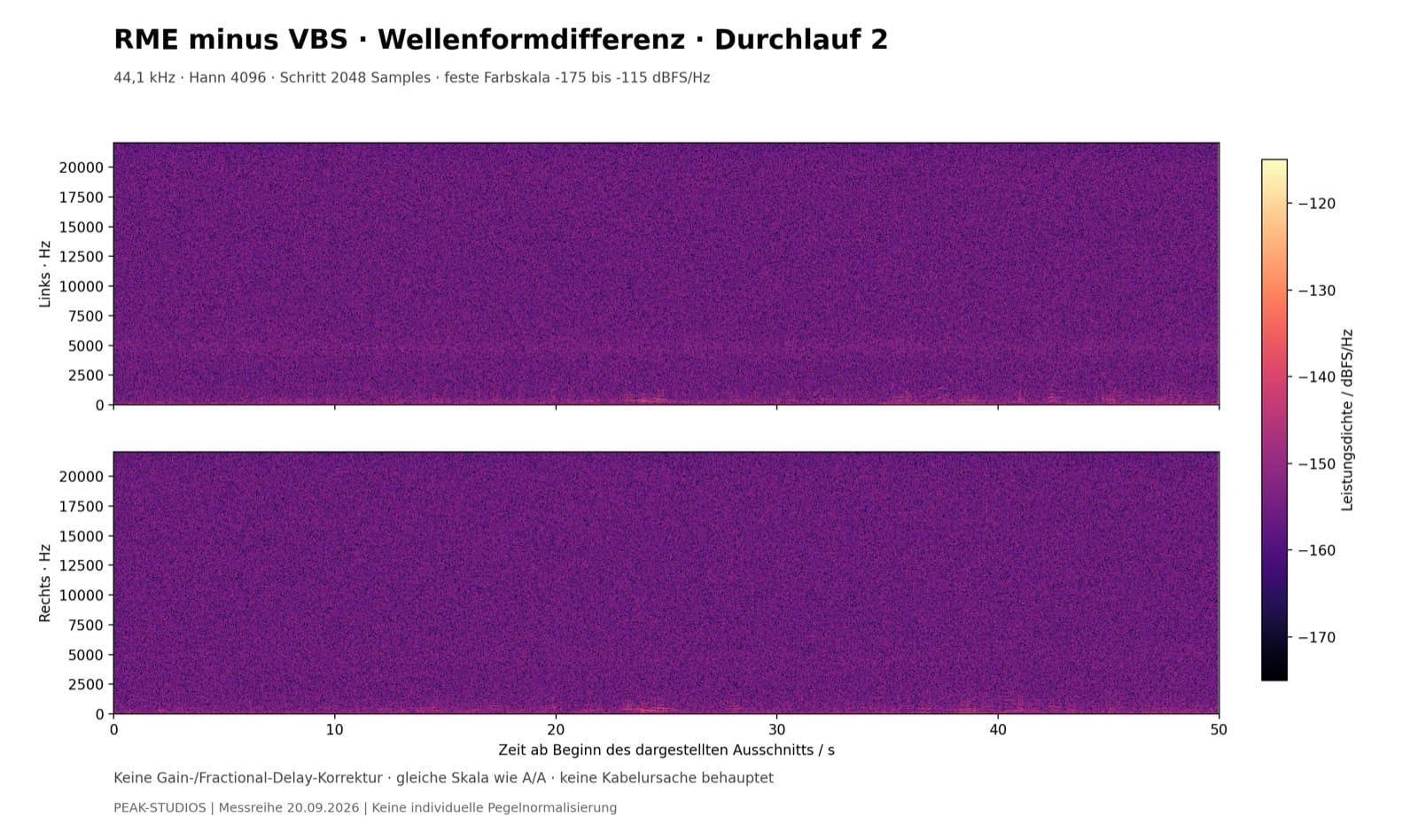
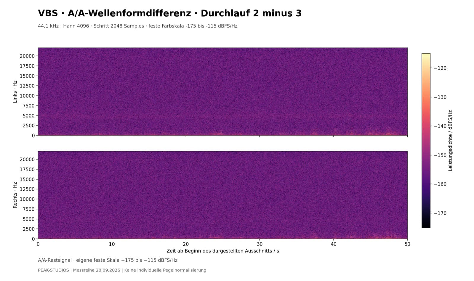
Cable sound difference spectrogram between VBS and RME conditions, uniform noise field without structure
Waveform difference between the two conditions, pass 2, inner section 50 s. Color scale fixed from −175 to −115 dBFS/Hz, no individual normalization. A uniform noise field without discernible structure is visible.
Difference spectrogram of two recordings under the same VBS condition as a measure of the repetition variation
For comparison on an identical scale: the difference between two recordings of the same Condition. Visually, practically the same finding – that's precisely the point. Without this benchmark, the image above would be impossible to classify.
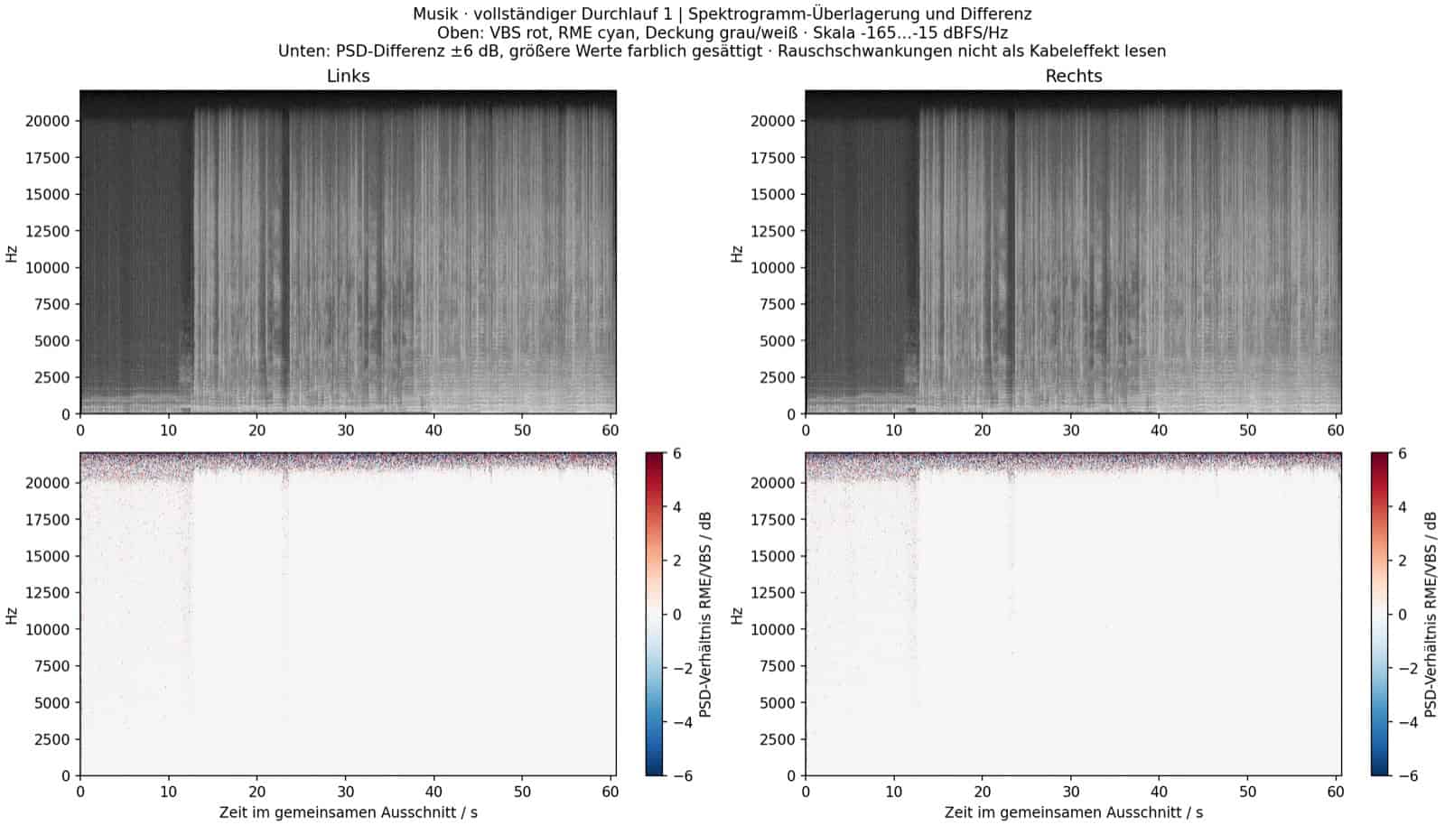
Spectrogram superposition of both cable conditions for the music signal with a difference card underneath.
Comparison of both conditions for the music signal: above are the superimposed spectrograms (VBS red, RME cyan, overlay gray to white), below is the power density ratio. The music signal appears consistently in overlay colors – the colored areas at the bottom are noise, not a cable signature.

Temporal stability – the jitter argument in cable sound

Because the word "jitter" is often mentioned in connection with digital connections, we examined the timing of the signals. Sixty individual tests (five take pairs × six windows × two channels) yielded results with a search range of ±4 samples. Everywhere an integer residual offset of zeroThe subsequent fine-tuning remained below 0,000024 Samples, the derived equivalent drift slope under 0,0000043 ppm.

Nevertheless, the following applies: These figures are model-based diagnostics – not a calibrated jitter measurement. They demonstrate that the comparison method does not require time correction. Anyone wanting a true statement about jitter needs a measurement procedure specifically designed for that purpose; we did not use one and therefore make no claims about jitter.

QUESTIONS ABOUT THE METHODOLOGY OR YOUR PRODUCTION?

Write to us – about this test, your setup, or your next song. We usually get back to you within 3 hours (on weekdays).

You can reach us by phone from Monday to Friday from 9 a.m. to 8 p.m.

Silence, sine wave and sweep: Cable sound measured in units of measurement

Measured variableVBS L / RRME L / Rdifference
Silence, 20 Hz–20 kHz, unweighted-113,619 / -113,681 dBFS-113,516 / -113,565 dBFS+0,104 / +0,116 dB
1 kHz fundamental frequency (RMS)-4,20712 / -4,18519 dBFS-4,20710 / -4,18518 dBFS+0,000024 / +0,000006 dB
Total harmonic distortion H2–H100,000299 / 0,000231%0,000301 / 0,000231%
THD including noise (THD+N)0,000584 / 0,000544%0,000576 / 0,000540%
Sweep transmission at 1 kHz-0,19737 / -0,17544 dB-0,19727 / -0,17535 dB+0,000103 / +0,000094 dB
Maximum deviation across 241 frequency support points <0,000163 dB

First, let's look at the frequency response: The curves overlap so closely across the entire audible range that they lie on top of each other in the diagram. The difference lies in... less than two ten-thousandths of a decibel – several orders of magnitude below what is discussed in practice.
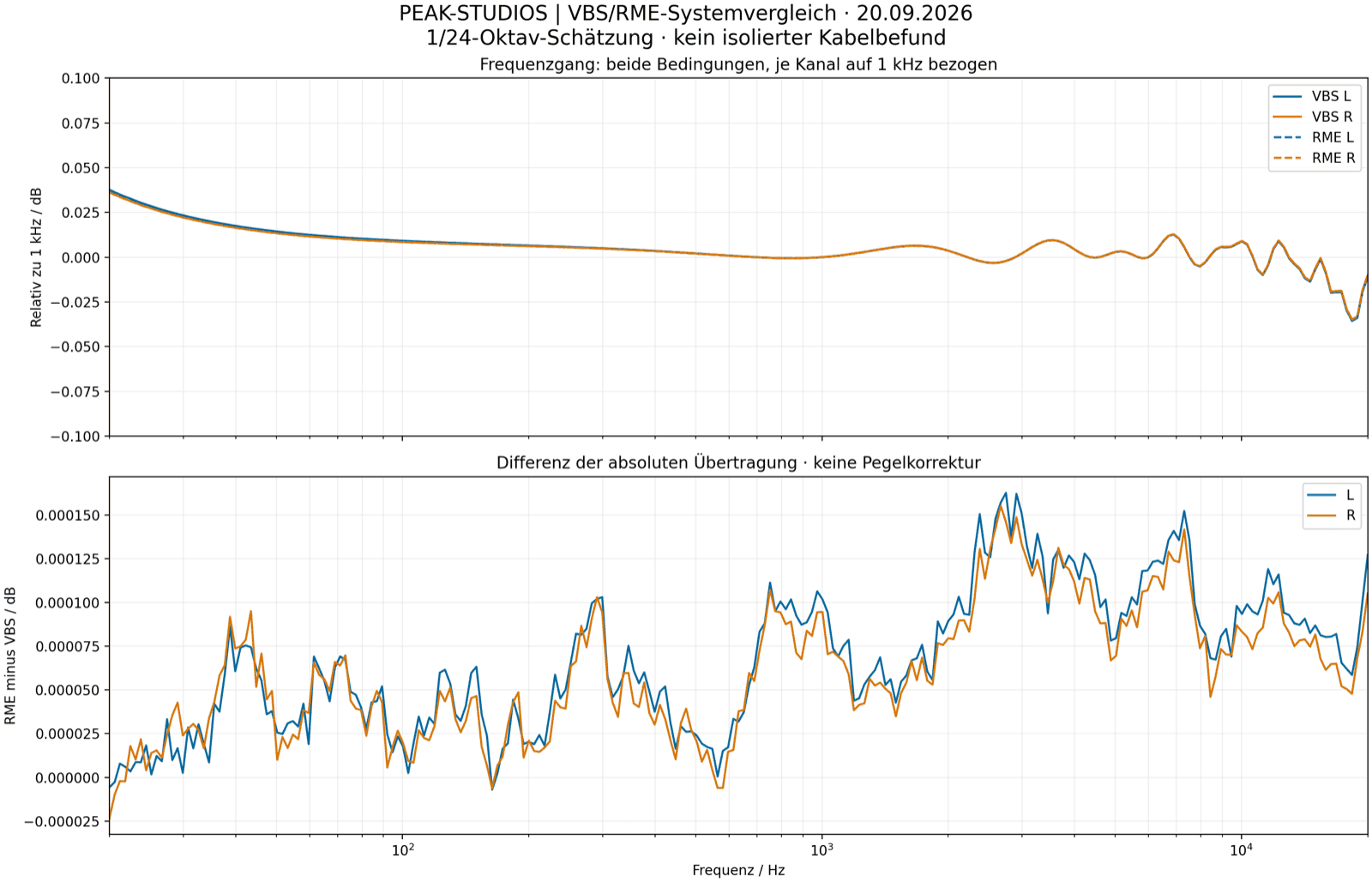
Cable sound measured: Frequency response of both USB cable conditions, the curves are identical.
Top: Frequency response of both conditions, referenced to 1 kHz per channel (1/24-octave estimation, 241 data points). Bottom: The absolute difference – please note the axis scale in ten-thousandths of a decibel.
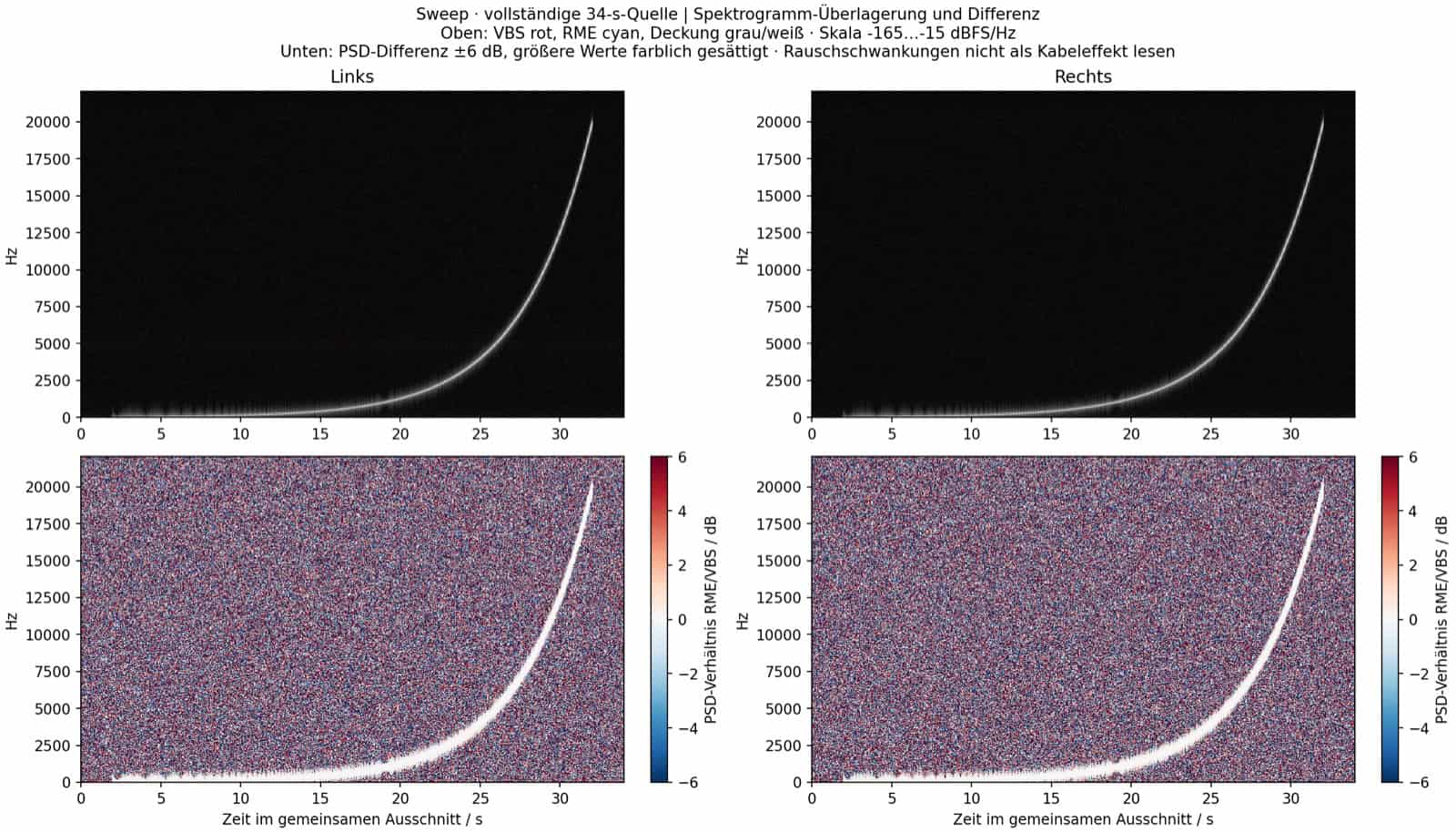
Spectrogram superposition of VBS and RME conditions during the sweep; the sweep line appears completely white.
The same comparison applies to the sweep. Above Both conditions overlap: VBS is colored red, RME cyan – where both are equally strong, this results in gray to white. The sweep line appears consistently white, meaning both states overlap across the entire frequency range. unten The power density ratio with a fixed scale of ±6 dB: The grainy pattern is noise that produces large relative values ​​in practically signal-free areas – it is not a cable signature.

One striking feature: noise level in silence.

However, the reference condition in the 20 Hz to 20 kHz band is approximately 0,10 to 0,12 dB higher. This is the only value in this measurement series that is noticeably above the noise floor. Before anything is done with this information:

  • There are only one still image per conditionNo repetition, no indication of variance, therefore no basis for attributing causes.
  • Both cables were replaced together. Even if the difference is real, it says nothing about it. which of the two compounds that caused it – or whether either of them caused it.
  • The state of clocking, internal signal processing, and input gain was not completely independently reread after the change.

Furthermore, 0,1 dB in the noise band of a system that has noise at −113 dBFS is far below what matters when music is playing.
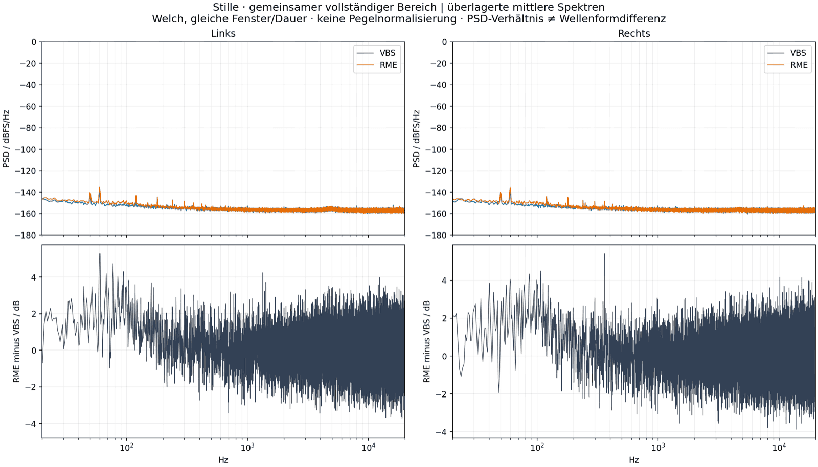
Cable sound in silence: Noise spectra of both conditions with mains hum pattern at 50 Hz and multiples thereof.
Silence in the shared inner window, superimposed mid-range spectra. The typical mains hum pattern at 50 Hz and its multiples is visible at the top – anyone who finds such lines in their own setup will Regarding the causes of hum in the audio signal find. Important regarding the lower curve: The difference fluctuates by several decibels per frequency band – this is normal behavior for random noise and no cable signatureA power density ratio is not a waveform zero test.
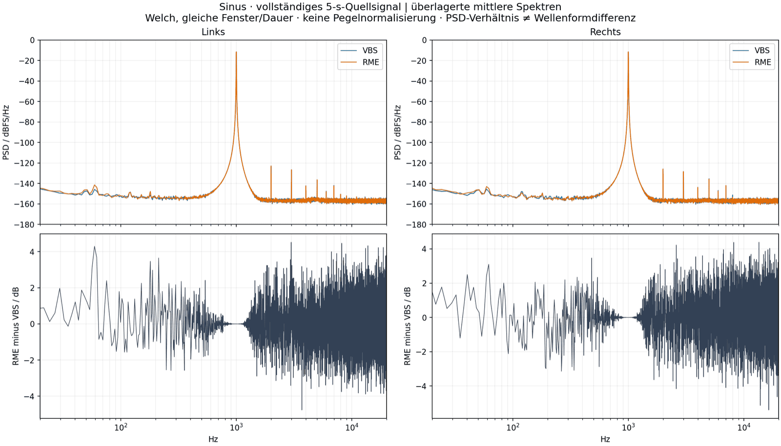
Superimposed spectra of the 1 kHz sine tone under both cable conditions with virtually identical harmonic patterns
The 1 kHz sine wave over its full length. The fundamental tone and harmonic patterns of both conditions are practically identical; the distortion values ​​are around 0,0003%.

Regarding the number of decimal places: Many of the values ​​above have five or six decimal places. That's the Computational solution of the procedureNot the measurement accuracy. We have not determined a calibrated measurement uncertainty for this chain. Anyone who makes a physical statement out of 0,000103 dB is overstretching the data.
Counter-test to the original: does cable sound affect loyalty?

Finally, we directly compared both conditions to the original digital file – that is, to what near the entire analog loop in the project was involved.

Waveform spacing from the originalVBS L / RRME L / R
at unchanged recording level-40,26948 / -40,52382 dBFS-40,26950 / -40,52380 dBFS
after pure level adjustment (diagnosis)-41,07187 / -41,12496 dBFS-41,07185 / -41,12497 dBFS

Why there is no stable winner

Initially without adjustment: The reference condition on the left is slightly closer to the original, the test condition on the right. After simple level adjustment. The order is reversed in both channels.The differences are approximately 0,000013 and 0,000023 dB respectively – and are therefore smaller than the variation shown by the same condition over its five runs (approximately 0,00017 to 0,00025 dB).

Consequently There is no clear winner here. Which condition is numerically closer to the original depends on which channel and level treatment are considered. This is not a result that can be unilaterally reversed.

Two numbers that are often confused

Furthermore, another classification that is often confused: The distance to the original is approximately -40 dBFS, the difference between the two recordings is approximately -110 dBFSThese are two completely different quantities. The -40 dB includes the entire common system transmission – level, phase, filter, conversion in both directions. That is no distortion from a cable, but rather what an analog loop simply does to a signal. Both states demonstrate this equally.

The blindfolded round: 11 to 9

However, measured values ​​don't answer the question that most people are actually asking. That's why we also listened – in a blinded manner.

Structure of the blind test

A test package was built from the recordings for this purpose: 20 fixed rounds, each with three files bearing the neutral identifiers A, B, and X. A and B represent the two states of the same recording pair, X is a byte-identical copy from A or B. Five pairs of recordings, each presented four times, order randomly shuffled, the assignment of A/B and X drawn independently each round.

Furthermore, the following applies to all 60 files: 50 seconds, stereo, 44,1 kHz, 32-bit float, same size, same format, metadata removed, modification time standardized. No level normalization. The assignment key was predefined using a checksum and was not visible until after the evaluation; the definition was subsequently verified unchanged, as were the checksums of all 60 files. Monitoring was not conducted using comparison software, but rather by neutrally switching tracks in a separate test project.

Preference or discernible sound? What was really asked about cable sound?

This report needs to be more honest than most cable tests online.

In all 20 rounds, participants were asked about their preference: "What is better, clearer, more resolving overall?" It was not The question asked: "Is X equal to A or equal to B?"

However, that is a crucial difference. The classic ABX question is a Identification task – it measures whether someone can reliably distinguish between two signals. What we have here is a Preference survey – it measures what someone prefers. Both are legitimate, but you mustn't sell one as the other.

For the sake of completeness: In an early analysis, a statement from Round 1 was incorrectly interpreted as a formal ABX response. This has been corrected. The original recording remains unchanged in the database; the outdated interpretation is marked as such.

The result of the cable sound test

Blinded preference trial: 20 rounds, one listener

The criterion in all rounds was: "better, clearer, more resolving overall" – not an identification task.

Expected probability of random occurrence: 10
11
9
VBS Audio Own55 percent of the winning elections
RME original cable45 percent of the winning elections

Two-sided exact binomial test against a fair 50:50 distribution: p = 0,824. This does not prove a systematic preference – and therefore, it is also not proof of sound equality.

My own impression during the run-through, from the voice memo:

“Basically, the decision was incredibly difficult, but I always have the feeling that with one signal, the voice or the midrange was generally more pronounced or boosted, and generally a bit clearer in context. Whether that's just my imagination, I obviously can't say for sure before we have the test results. […] The signals are fundamentally very, very similar in their sound characteristics.”

By the way: Whether your own studio knowledge is really as confident as it feels can be tested even without a listening comparison – our Knowledge quiz about mixing and mastering It asks questions from everyday studio life and proves more difficult than expected for most.

This is a personal impression from listening – and it's written here exactly as it was heard. It is no measurement resultAnd it is not reinterpreted as one here. When it clashes with the numbers, neither the numbers nor the impression gain: Then both stand side by side, just as they do now.

What the statistics say – and what they don't –

Therefore, to evaluate the results, one asks a simple question: If there were no difference in the evaluation and every choice was pure chance – how often would a result emerge that is at least as skewed as 11:9?

This can be calculated precisely. The null model is a fair 50:50 allocation – the blind draw produces exactly that. The event of interest is a deviation of 10:10. in any direction, so at most 9 or at least 11 choices for one condition. Two pages because no direction was predetermined – we didn't predict which cable would win.

The result: p = 0,824.

To put it simply: By pure chance, an outcome at least as unbalanced would occur in approximately 82 out of 100 such series. 11:9 is therefore a completely unremarkable random result. Additional measurements were taken for verification. one million series simulatedOf these, 823.938 were at least as unbalanced, i.e., 82,3938% compared to exactly 82,3803% – with a simulation error of approximately 0,038 percentage points. The simulation confirms the calculation; it generates no additional audio material and does not increase the sample size. The calculations were performed using the exact binomial test from SciPy, cross-checked with an independent calculation.

Four misinterpretations to avoid when dealing with p-values

Experience shows that this value is regularly reported incorrectly. It explicitly does not mean:

  • Not "The cables sound the same with 82% probability." A p-value is not a probability for a hypothesis.
  • Not "82% of the answers were guesses." The value says nothing about individual answers.
  • Not "55% success rate". There were no right or wrong answers because it was not an identification task.
  • Not "This proves that there is no difference." Non-significance is not proof of equality.

And the point that is most often overlooked: Two audibly different versions can still be preferred equally often. An 11:9 ratio is compatible with indistinguishable signals – but equally so with distinguishable signals without a stable preference. Both possibilities remain open after this pass.

The limitations of this cable sound listening test

  • A listener. No statement about other ears.
  • A piece of music. No statement regarding other materials.
  • Five pairs of recordings, listened to four times. These are repetitions of the same recordings, no 20 independent hardware changes.
  • Both cables were replaced together. No isolation of individual connections.
  • Not a standards-compliant ABX or ITU test. We do not claim conformity to any standard; the Methodological framework of ITU-R BS.1116-3 This is only for contextual purposes.
  • The playback settings were not independently logged during listening. Import, fader, pan, effects, and output assignment are not independently documented. A subsequent review of the project cannot retrospectively prove its original state.
  • An observation we cannot argue away: In round 1, B and X were byte-identical but described differently. In a pure preference query, this isn't a wrong answer – but it shows how much perception can fluctuate when signals are very similar. The cause cannot be determined from the responses.

Cable sound in conclusion: what that means – and what it doesn't.

What we can say about cable sound

In summary: Under the conditions documented here – this studio, these devices, this piece of music, this listener – both states delivered virtually identical signal transmission. In the tested digital excerpts, the data arrived flawlessly at the 24-bit level. The blinded preference test showed no systematic advantage. And no consistent ranking emerged compared to the digital original.

What we cannot say

  • That audiophile USB cables cannot have any influence whatsoever. This test examines two specific cables in a specific chain – not the principle.
  • That the differences are inaudible. This would require an identification task, which we did not perform.
  • The slight noise variation during silence is due to the cable. However, one silent recording per state, with both connections switched simultaneously, does not establish causality.
  • The manufacturer's claims regarding microstructure, geometry, and time behavior are incorrect. They are simply not compatible with this design. Not checked.

Fair to the manufacturer

Andrej, at least, gave his prior written consent to the entire procedure – blinded hearing test, objective measurements, long-term observation – even though it was clear that we would also publish a negative result. He provided the cables free of charge and approved the publication without influencing the outcome. This is more transparency than is customary in this industry, and it belongs in this report just as much as the figures.

Fair in relation to the question

Otherwise, if we truly wanted to answer the question "Can the states be reliably distinguished by sound?", we would need a separate identification series with a predefined evaluation and a sampling plan tailored to the effect we want to find. We deliberately omitted this – you don't repeat a test until the desired result appears.

What I personally take away from this

Two things.

First: The effort was definitely worthwhile – not because of the result, but because of the method. The repeat comparisons were the most important part of this measurement series. Without them, I would have seen a residual difference of −109,6 dBFS between the states and probably thought that was significant. Only the measure of "how much does the same system fluctuate with itself?" makes the number meaningful. Anyone who publishes such tests without this step is publishing their own noise.

We offer precisely this principle – check first, then decide – as a service: In the case of a mix analysis We listen to a production in detail and identify where its real potential lies. And anyone who wants to know what our mastering will do to a specific song before an entire album is produced can find out with a single song as a test mastering Find out – a verifiable result instead of a promise.

Why blind listening is uncomfortable

Secondly: While listening, I definitely thought I heard something – clearer midrange, a bit more resolution. After the blinding was lifted, it showed 11:9. This is precisely the experience one needs to have to understand why blind listening is so uncomfortable and yet so necessary when dealing with small differences.

Ultimately, what remains is a simple recommendation for anyone facing the same question: Before investing four-figure sums in a connection, it's worth taking a look at where the real leverage points lie within your own setup. Based on that, what a complete mixing and mastering production costsThe price of a single cable is already disproportionate to its demonstrable benefit. Room acoustics, listening environment, and the quality of the recording itself In our daily work, we deal with magnitudes that we are discussing here in ten-thousandths of a decibel. Even a cleanly configured audio computer It provides more stability in everyday use than any cable.

Methods and data appendix for cable sound measurement

Finally, this section is for anyone who wants to recalculate or replicate the project. Those who only wanted the result can find it above.

Recording and music comparison

Format: 44,1 kHz, stereo, 32-bit float. Music source: 2.675.375 samples (60,666099773 s). Raw music file: 317,875873 s or 320,259524 s, five complete passes extracted each – integer trimming only, no processing.

Music comparison: Identical inner section 5–55 s. Error level = RMS of the direct waveform difference. No gain, tone, fractional sample, or resampling correction. 25 cross-comparisons, 10 repetition comparisons per condition.

Test signals: Silence, sine wave and sweep

Silence: common inner window 1–28,889 s. Welch method, 2-s Hann window, 50% overlap, mean distance per window, band 20 Hz–20 kHz, unweighted (no A rating).

1 kHz sine wave: Identical file window 2–5 s. Frequency adjustment of the fundamental tone, least-squares fit, harmonics H2 to H10. Total harmonic distortion including noise from the fundamental-corrected remainder in the band 20 Hz–20 kHz. A method check with a synthetic signal of known distortion (0,1% second harmonic) yielded −60,000005 dBc compared to a target value of −60 dBc.

sweep: Source 34 s total (2 s silence + 30 s logarithmic sweep 20 Hz–20 kHz + 2 s silence), peak level −18 dBFS, fade-in/fade-out times 50 ms and 20 ms respectively, both channels identical. Both feedback loops referenced to the same complete source. Identical FFT processing, quotient of summed spectral powers in 1/24-octave bands, 241 support points, absolute and additionally referenced to 1 kHz per channel. A synthetic control with a known gain difference of −6 dB was passed. The edge bands are interpretable to a limited extent due to fade-in/fade-out times and sweep limits; a harmonic-resolved distortion measurement across the frequency range was therefore not performed.

Spectrograms and why difference images can be misleading

Procedure: Short-time Fourier transform with symmetrical Hann window 4096, step size 2048, no mean removal, one-sided power density in dBFS/Hz. Main scale −165 to −15 dBFS/Hz; noise and residual signal views separately −175 to −115. Overlays with common scale, no individual normalization. Welch comparisons: Hann 16384, at silence 65536, 50% overlap. Spectrogram definition from SciPy is the basis of the presentation.

Why difference images should be read with caution: A difference map of the form 10·log₁₀(power density A / power density B) is no spectrogram of a waveform differenceRandom noise is never identical in every frequency band; in areas with very low absolute levels, this results in large relative deviations that appear colorful but are meaningless. Therefore, this article includes the absolute scale and this explanation with every such graph.

What the test doesn't say about cable sound

All values ​​mentioned in the text are taken from the archived evaluation files of the measurement runs and were checked against these files and their respective evaluation windows for the purposes of this article. A complete source and statement register, which traces each figure back to the file, window, and procedure, is available in the project archive.

What cannot be determined from this data: Crosstalk between the channels (the excitation was identical on both channels), calibrated jitter, isolated electrical cable characteristics, and any statement about devices, rooms, music, or listeners outside of this setup.

Conflict of interest and data holdings

The cables tested were provided free of charge as product samples and remain with Peak-Studios. No money changed hands, there were no content specifications, and the manufacturer did not approve this text. The manufacturer agreed to the procedure and the publication of a null result in advance.

Raw recordings, blind test packages, answer keys, and evaluation scripts are fully archived and protected against alteration via checksum manifests. They are not publicly available due to copyright restrictions on the test music and test integrity. We are happy to answer any questions regarding the methodology directly.

Frequently asked questions about cable sound

Not during the data transmission itself – that is error-protected. Entweder kommt ein Paket korrekt an oder es kommt gar nicht an. Diskutiert werden deshalb meist indirekte Wege: Masseführung, Schirmung und Einstreuungen in die analoge Umgebung. Unser Test hat beides geprüft: die Datenübertragung (auf 24-Bit-Ebene fehlerfrei) und die analoge Ausgabe (praktisch deckungsgleich). Er beantwortet die Frage damit aber nur für diese zwei Kabel in dieser Kette.

In our series of measurements, no cable sound was detectable with USB. This cannot be answered in general terms because "digital audio cables" refers to four different transmission methods. With USB in asynchronous mode, the device itself provides the clock signal – any influence from external sources is technically difficult to explain and was not detectable in our measurements. With AES3, coaxial S/PDIF, and Toslink, the clock signal is embedded in the signal; here, impedance errors and reflections can indeed have measurable effects. Our test covers only the USB connection.

The issue lies in dropouts, crackling, and increasing error counters – not in a change in timbre. Dazu kommen Verbindungsabbrüche. Viele Audiointerfaces zeigen die Fehlerzähler des Treibers direkt an. Steht dort dauerhaft null, arbeitet die Strecke im geprüften Bereich fehlerfrei.

Because this round asked about preference, not identification. Das im Nachhinein als ABX zu verkaufen, wäre unredlich. Für eine belastbare Aussage über hörbare Unterscheidbarkeit bräuchte es eine eigene Serie mit vorab festgelegter Auswertung und passender Stichprobenplanung.

Questions about test design and validity

No – with 20 random decisions, 11:9 is a completely unremarkable result. Es tritt unter reinem Zufall in rund 82 von 100 Fällen mindestens so ausgeprägt auf. Aus 11:9 lässt sich kein Vorteil ableiten.

Aus praktischen Gründen im laufenden Studiobetrieb – und weil der realitätsnahe Vergleich der Auslieferungszustand gegen den Testzustand ist. Der Preis dafür ist, dass die Ursache eines etwaigen Unterschieds nicht einer einzelnen Verbindung zugeordnet werden kann. Diese Einschränkung steht deshalb an jeder relevanten Stelle im Text.

Only to a limited extent – ​​measurements were taken on a specific chain with specific devices. Andere Interfaces, andere Masseverhältnisse und andere Räume können sich anders verhalten. Die Methode ist übertragbar – das Ergebnis nur als Hinweis.

They represent the computational resolution, not the measurement accuracy. Eine kalibrierte Messunsicherheit für diese Kette haben wir nicht bestimmt. Deshalb interpretieren wir Unterschiede nur dann, wenn sie größer sind als die beobachtete Streuung derselben Bedingung.

Technical terms and practice

dBFS is the digital level relative to full output: 0 dBFS is the maximum, all values ​​below it are negative. Die Abkürzung steht für „Dezibel relativ zur Vollaussteuerung“. Ein Restsignal von −110 dBFS ist also extrem leise – rund 110 Dezibel unterhalb der Vollaussteuerung.

Beim Nulltest zieht man zwei Signale voneinander ab; bleibt exakt Stille übrig, sind sie identisch. Das funktioniert bei rein digitalen Kopien. Sobald ein Signal durch Digital-Analog- und Analog-Digital-Wandlung läuft, bleibt immer ein Rest – Wandlerrauschen und minimale Schwankungen. Deshalb braucht man zusätzlich den Vergleich einer Bedingung mit sich selbst als Maßstab.

Auf Raumakustik, Abhörsituation und die Qualität der Aufnahme selbst – in dieser Reihenfolge. Das ist die Erfahrung aus unserer täglichen Arbeit. Diese drei Punkte bewegen Größenordnungen, über die in Kabeldiskussionen in Zehntausendstel Dezibel gestritten wird.

Image by Chris Jones

Chris Jones

CEO – Mixing and Mastering Engineer. Founder of Peak-Studios (2006) and one of the first online service providers for professional audio mixing and mastering in Germany.